How the methods work, what the experiments show, and where the results apply.
01 / 2023 / IEEE Transactions on Computational Imaging
Monotone operator learning
Learned MRI reconstruction with lower training memory and explicit stability constraints.
The problem
Unrolled reconstruction networks store intermediate states during training. As the number of iterations or image dimensions grows, this memory cost can prevent joint reconstruction of 3D or dynamic MRI.
The approach
Alternate a learned image update with a step that fits the acquired MRI measurements.
Constrain the learned operator to control how the reconstruction responds to changes in its input.
Run the reconstruction to a fixed point and train through that equilibrium, without storing every iteration.
The method in the paper
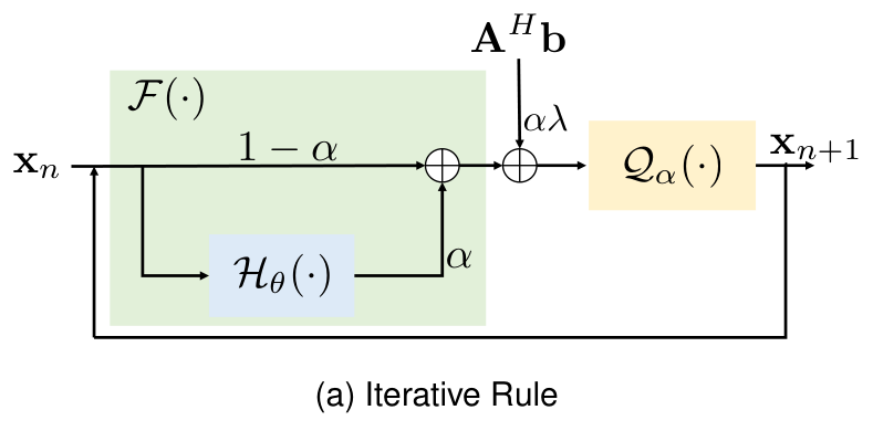
Figure 1(a). The original iterative rule. Hθ is the learned CNN; Qα is the data-consistency operation. The loop repeats until the reconstruction reaches an equilibrium.Open full-size figure ↗Figure in the paper ↗Swipe across wide figures to compare panels.
What the experiments show
The paper reports approximately 10× lower training memory than ten-iteration unrolled networks, with comparable reconstruction quality in its 2D MRI experiments. This reduction also enables a demonstration that reconstructs cardiac cine MRI jointly across time.
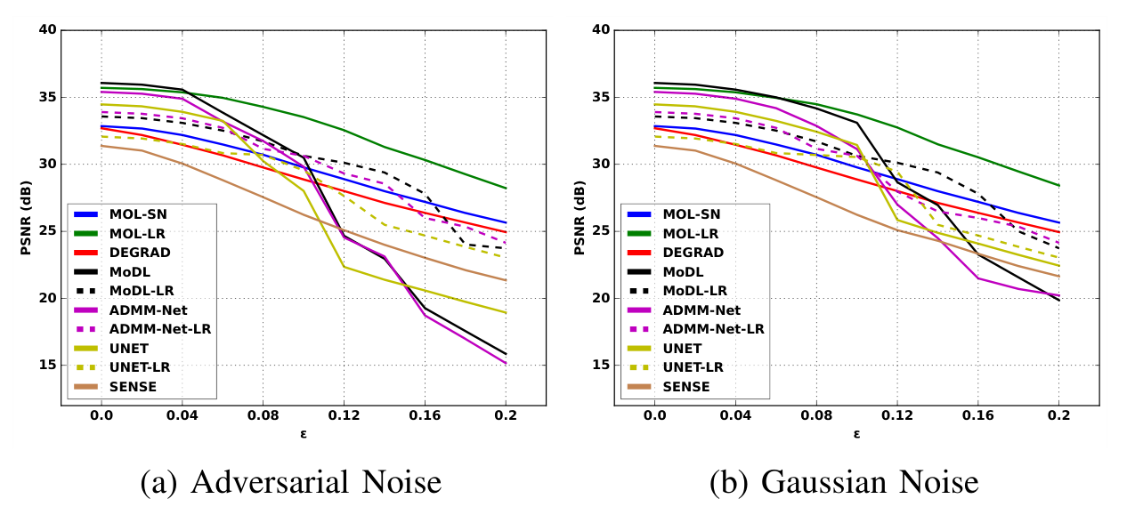
How to read the figure. Follow the green MOL-LR curve in the left plot. It loses image quality gradually as adversarial perturbations increase, while several unconstrained models drop sharply. The right plot provides the corresponding Gaussian-noise comparison.
Figure 7. Reconstruction quality as measurement perturbations increase. The horizontal axis is perturbation size relative to the measurements. The vertical axis is PSNR in decibels; higher is better.Open full-size figure ↗Figure in the paper ↗Swipe across wide figures to compare panels.
Scope of the result
Formal uniqueness, convergence, and robustness guarantees require the strict monotone constraint. MOL-LR uses an approximate constraint: its strong reconstruction and robustness results are empirical, rather than the same strict guarantee.
02 / 2023 / IEEE Transactions on Medical Imaging
ENSURE: learning without clean reference images
Train a reconstruction network from incomplete, noisy MRI measurements.
The problem
Supervised learning normally needs a clean, fully sampled target image for every training example. Such targets can be expensive or impractical to acquire in MRI. Simply fitting noisy measurements can also teach a network to reproduce the noise.
The approach
Use an ensemble of sampling patterns across training examples to expose different parts of the image information.
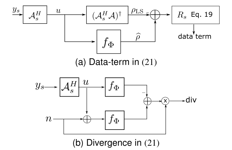
Combine a weighted data term with a noise-aware divergence term to estimate reconstruction error without clean targets.
Train the reconstruction network end to end using this estimated risk.
The method in the paper
Figure 1. The two components of the ENSURE training loss: a data term and a divergence term. The divergence correction accounts for measurement noise; the weighting accounts for how samples are acquired.Open full-size figure ↗Figure in the paper ↗Swipe across wide figures to compare panels.
What the experiments show
Across the reported MRI experiments, ENSURE approaches supervised reconstruction quality while training without fully sampled, noise-free targets. Its advantage over several other unsupervised losses becomes more pronounced at higher acceleration or noise.
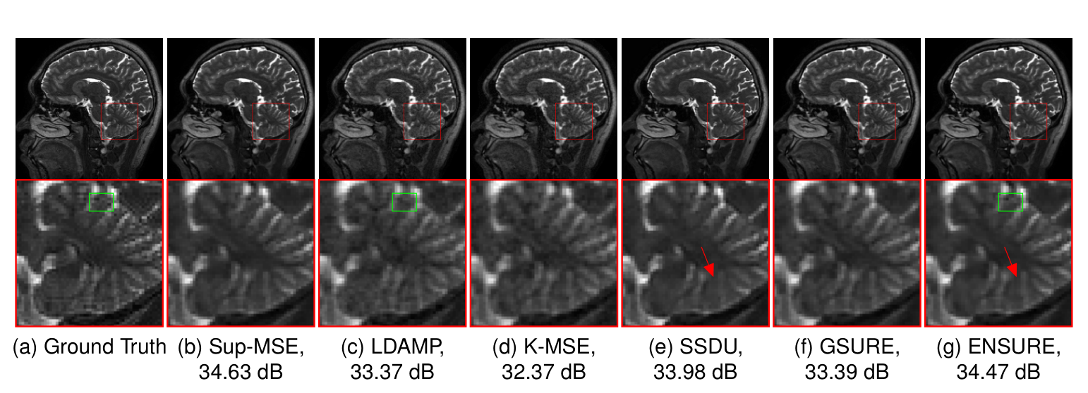
How to read the figure. Compare panel (g), ENSURE, with panel (b), supervised MSE, and the reference in panel (a). ENSURE preserves the fine structure indicated by the red arrow. The PSNR for this slice is 34.47 dB for ENSURE versus 34.63 dB for supervised training; higher is better.
Figure 4. Sixfold-accelerated brain MRI from a test slice. Ground truth is on the left; supervised training is panel (b), and ENSURE is panel (g). The bottom insets enlarge the cerebellum.Open full-size figure ↗Figure in the paper ↗Swipe across wide figures to compare panels.
Scope of the result
The loss relies on noise-variance estimation and adequate sampling coverage across the ensemble. Fully sampled images were retained for evaluation, although ENSURE did not use them as clean training targets. Reconstruction quality depends on the noise and sampling setting.
03 / 2020 / IEEE Transactions on Medical Imaging
Deep-SLR: fast calibrationless parallel MRI
Learn structured MRI relationships once, then reuse them during reconstruction.
The problem
Structured low-rank methods can recover MRI data without explicit coil-sensitivity calibration, but repeatedly estimating their filters from each scan is expensive. The challenge is to retain this structure with a much faster reconstruction.
The approach
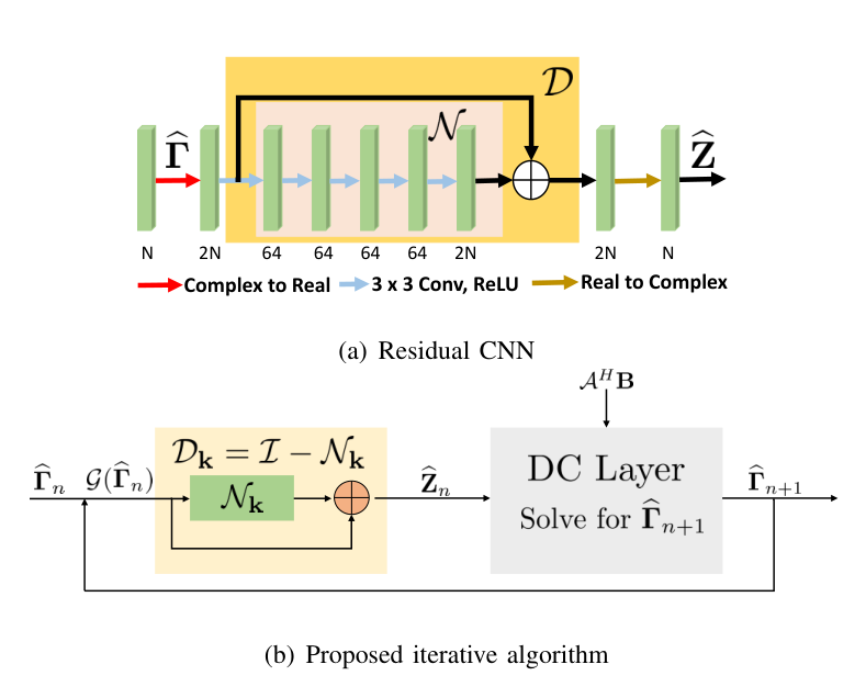
Learn a nonlinear filterbank in k-space, the frequency domain where MRI measurements are acquired.
Alternate the learned filtering with a step that fits the measured data, sharing network weights across iterations.
Add a complementary image-domain CNN in the hybrid H-DSLR variant to capture local anatomical structure.
The method in the paper
Figure 2. The original k-space Deep-SLR network. A pretrained residual CNN replaces repeatedly estimated linear filters, while the data-consistency layer retains the measurement model. The hybrid variant also adds an image-domain prior.Open full-size figure ↗Figure in the paper ↗Swipe across wide figures to compare panels.
What the experiments show
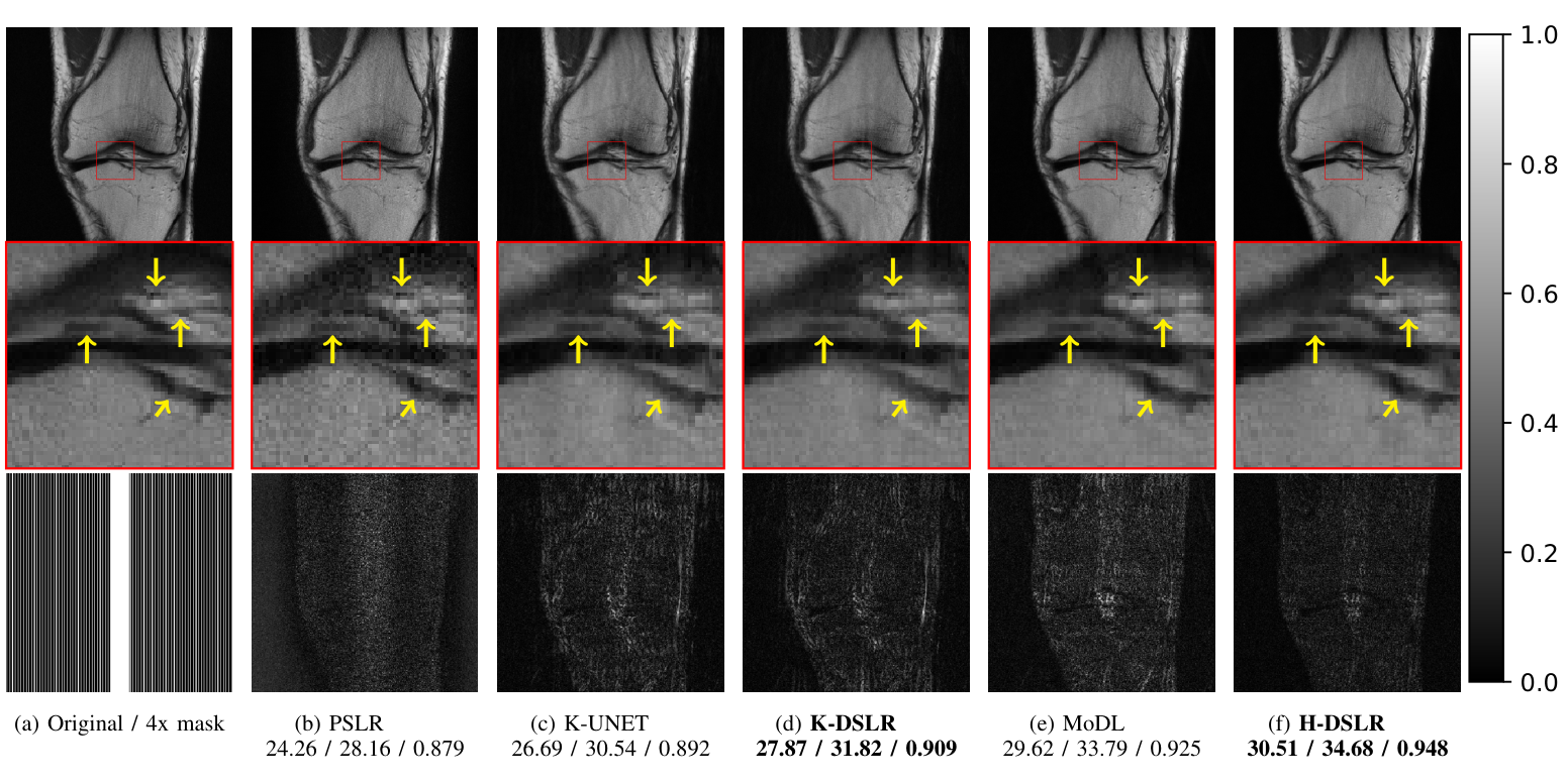
The hybrid method improves reconstruction quality over the k-space-only variant in these comparisons. Prelearning the filters also produces a runtime reduction of several orders of magnitude relative to the iterative structured low-rank benchmarks reported in Table II.
How to read the figure. Compare the yellow-arrow cartilage details in K-DSLR, panel (d), and hybrid H-DSLR, panel (f). Adding the image-domain prior reduces the remaining artifacts and better preserves the small structures. The error maps make the differences easier to see.
Figure 6. Fourfold-accelerated, 15-channel knee MRI. Top: reconstructions. Middle: enlarged cartilage regions. Bottom: sampling mask or reconstruction error. K-DSLR and H-DSLR are the proposed methods. Numbers below the panels are SNR / PSNR / SSIM; higher is better.Open full-size figure ↗Figure in the paper ↗Swipe across wide figures to compare panels.
Scope of the result
Calibrationless means that explicit coil-sensitivity maps are not needed. The paper evaluates brain and knee datasets and simulated calibration mismatches; it does not establish immunity to every kind of motion or distribution shift.
04 / 2025 / Journal of Nondestructive Evaluation
Plug-and-play reconstruction with a 2.5D prior
Use neighboring CT slices to preserve small internal defects in sparse-view scans.
The problem
Fewer X-ray views can shorten industrial CT acquisition, but the resulting artifacts can hide or distort small pores. A 2D prior processes each slice independently and misses information shared by neighboring slices.
The approach
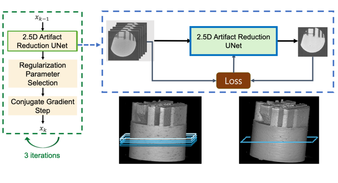
Feed five neighboring slices to an artifact-reduction network that estimates the center slice.
Alternate the multi-slice prior with a conjugate-gradient step that fits the X-ray measurements, using adaptive regularization.
Evaluate both image quality and whether the reconstructed volume preserves pores for defect detection.
The method in the paper
Figure 1. “2.5D” uses neighboring 2D slices as channels, rather than a full 3D CNN. The blue box shows prior training. The green loop combines that prior with the measurement model during reconstruction.Open full-size figure ↗Figure in the paper ↗Swipe across wide figures to compare panels.
What the experiments show
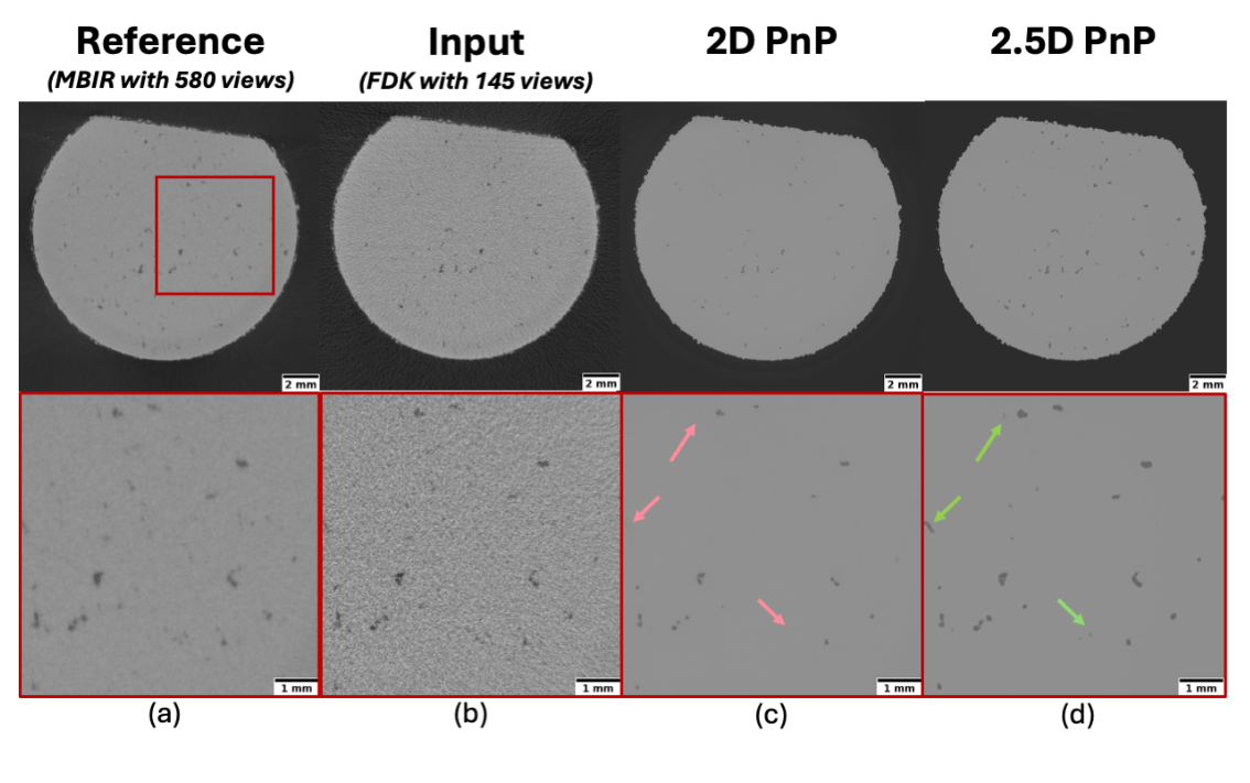
In this experimental scan, the prior trained on simulated data transfers to real measurements and improves pore recovery. The paper’s segmentation and precision–recall evaluations test whether the improved appearance translates into better defect detection.
How to read the figure. Compare the lower-row pores in 2D PnP, panel (c), and 2.5D PnP, panel (d), against the reference in panel (a). Pink arrows mark pores that the 2D prior misses or distorts; green arrows show structures better recovered with the multi-slice prior.
Figure 10. Experimental aluminum–cerium CT. Reference: MBIR using 580 views. Input and both PnP methods: 145 views. The lower row enlarges the same pore region; scale bars remain in the original figure.Open full-size figure ↗Figure in the paper ↗Swipe across wide figures to compare panels.
Scope of the result
The experimental comparison slightly favors 2D PnP on overall error and similarity scores (NRMSE and SSIM), while the 2.5D prior better preserves pores. In the very sparse 73-view tests, higher recall (more defects found) comes with lower precision (more false positives).
05 / 2019 / IEEE International Symposium on Biomedical Imaging
O-MoDL: learned priors in Fourier space
Combine continuous-image structure with learned Fourier-domain filtering and measured-data consistency.
The problem
Off-the-grid reconstruction exploits relationships implied by a continuous, piecewise-smooth image model. Traditional algorithms estimate these relationships iteratively, which is computationally demanding.
The approach
Start with the off-the-grid GIRAF formulation, which alternates filtering and measurement-consistency steps.
Replace its linear Fourier-domain denoiser with a CNN learned from example MRI data.
Reuse the learned block across iterations, while retaining the explicit MRI forward model.
The method in the paper
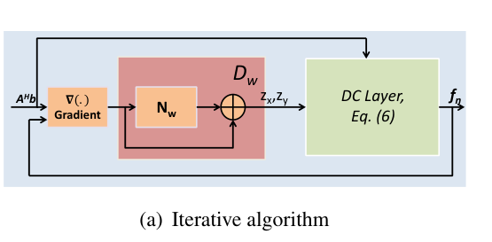
Figure 1(a). Cropped from the original iterative algorithm. The learned residual block Dw filters Fourier coefficients of image derivatives; the DC layer fits the acquired measurements. The full Figure 1 compares GIRAF and O-MoDL denoiser architectures.Open full-size figure ↗Figure in the paper ↗Swipe across wide figures to compare panels.
What the experiments show
The preliminary experiments demonstrate improved reconstruction over an image-domain MoDL network trained with the same number of iterations and parameters. The paper reports about 50 milliseconds to reconstruct a single image on its experimental setup.
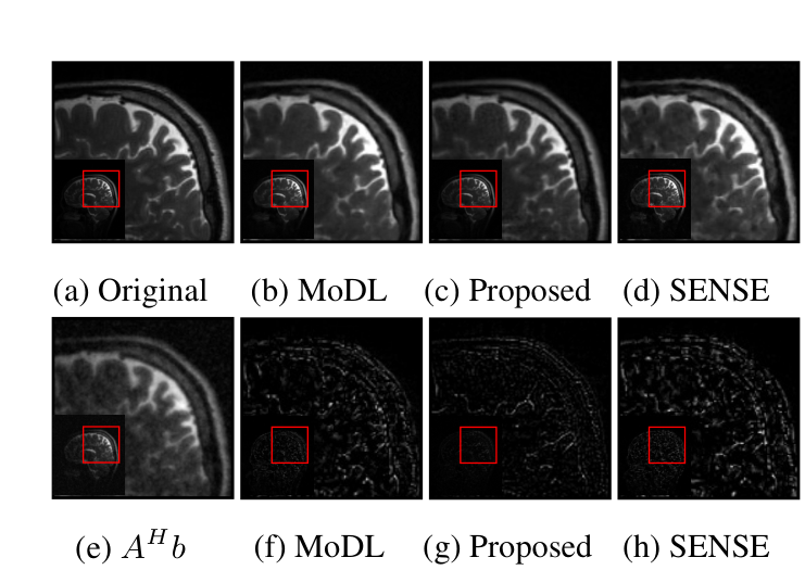
How to read the figure. Compare “Proposed” in panel (c) with MoDL in panel (b), then compare their error maps in (g) and (f). This example reports SNR of 13.84 dB for O-MoDL versus 12.58 dB for MoDL; higher is better. SNR is different from the PSNR metric used in the other MRI examples.
Figure 3(a–h). Cropped to the first coil example at fourfold acceleration. Top: original image, MoDL, proposed O-MoDL, and SENSE. Bottom: zero-filled input in (e), then error maps for the three reconstructions in (f–h).Open full-size figure ↗Figure in the paper ↗Swipe across wide figures to compare panels.
Scope of the result
Training used four subjects, with a fifth subject held out for testing. The experiments reconstruct individual coil images; the paper leaves joint multi-coil reconstruction and broader validation for future work.